
Written by: Corey Hoffstein | Newfound Research
Summary
- Since 2009, any decision to de-risk in a trend equity portfolio has largely been the wrong decision.
- At the time of writing, we implement a 1-month tranching process in most of our trend mandates, which has the effect of dollar-cost averaging signal changes over a 1-month period.
- We adopted this approach for a number of reasons, including: (1) to align our rebalance frequency with what we believe to be the optimal forecast horizon for trend following; (2) to exploit short-term mean-reversion in our portfolios; and (3) to modulate portfolio positioning conviction based upon signal consistency.
- Given the speed of the March 2020 sell-off, we’ve received a number of questions about this choice and whether simply implementing trend signals immediately would be more effective.
- In this note, we briefly explore this question and find that, empirically, the choice to tranche has been superior for a meaningful number of asset classes over the last 30 years.
- Finally, we demonstrate that tranching choices can be thought of as a means of placing weight on prior signals and that combining different tranching speeds in the same portfolio can create non-linear reaction functions.
In the 2008 comedy Forgetting Sarah Marshall, Peter Bretter (played by Jason Segel) takes a vacation to Hawaii in an attempt to get over his ex-girlfriend (played by Kristen Bell).
In one of my favorite movie scenes ever, he decides to take surfing lessons from Kunu (played by Paul Rudd).
Now, if you’ve never taken a beginner’s surfing lesson, it’s important to know that they start on the beach. The instructor teaches the student how to actually stand up on the board, which is a not-so-trivial action.
“Don’t do anything,” Kunu says sagely. “The less you do, the more you do. Let’s see you pop it up.”
Peter jumps up on the board.
“That’s not it at all,” Kunu says disapprovingly. “Do less. Get down. Try less. Do it again.”
Peter tries to get up much slower, but before he even gets off his stomach, Kunu says, “Nope, too slow. Do less.”
Peter begrudgingly resets and tries again. This time, he gets to his knees before Kunu chimes in. “You’re doing too much. Do less. Pop down.”
“Remember, don’t do anything,” Kunu instructs. “Nothing. Pop up.”
To which Peter finally does nothing.
“Well, you… no, you’ve got to do more than that. Because you’re just lying… it looks like you’re boogie boarding.”
As trend followers, we can sympathize with Peter. For the last decade, “You’re doing too much. Do less,” has been the best course of action. Until March, when it became: “Well, you … no, you’ve got to do more than that.”
Specifically, we have received many questions relating to our method of tranching in our trend-driven strategies.
In most of our mandates, we specify a one-month tranching period, which means that if a trend signal turns off and stays off, the corresponding position will be reduced in size over the next month.
When faced with one of the fastest equity market declines in U.S. history, a month can feel like an eternity. “Well, you… no, you’ve got to do more than that.”
Some Intuition Behind Tranching
A one-month tranche can really be interpreted as saying, “we want a one-month holding period but we want to diversify our rebalance timing luck.”
But why would we want a one-month holding period? Why wouldn’t we just implement all our trend signals as soon as they change? To this, there are several answers.
Signal Forecast Horizon
One of the questions it is important to ask ourselves is, “what is this signal actually telling us?” When we say, “value is a slow-moving signal,” or “momentum is a fast-moving signal,” what does that mean?
It tells us something about how quickly we need to refresh our signals for them to remain relevant. Which, in turn, tells us something about the horizon over which those signals are relevant. For example, valuation signals provide almost no information about short-term market returns but can provide quite meaningful information about returns over the next decade. Conversely, trend may tell us something about short-term market probabilities, but little about what will unfold over the coming years.
If we evaluate and fully implement quantitative signals every day, we are effectively saying that we believe the optimal forecast horizon is one day. But what if we think a trend signal maximizes its informational accuracy over the next month?
For example, if our trend signal turns off today, we might believe that the conditional probability of tomorrow’s return still reflects a coin flip, but the conditional cumulative return over the next month has a higher probability of being negative.
So how would we square this up if yesterday’s signal is positive and today’s signal is negative? In theory, those forecast horizons overlap significantly. Do we ignore yesterday’s forecast?
Tranching allows us to express a view about the optimal forecast horizon.
Lead/Lag Effects of Trend and Mean-Reversion
Empirical evidence suggests that trend and mean-reversion often lead and lag each other at different time horizons. A well-known example of this effect is in cross-sectional equity momentum, where the most recent month’s return is often ignored as short-term returns exhibit mean-reversionary tendencies.
Similarly, just as slower-moving trend signals change, short-term returns can exhibit mean reversion. Tranching may help a strategy capture these effects. For example, if the equity market sells off and trend signals turn negative, tranching may help the strategy sell into strength as the market exhibits short-term reversion.
This may also help reduce the impact of whipsaw.
Signal Certainty
Another important aspect to consider is signal confidence. Consider a simple signal that changes when price crosses above or below its 200-day moving average. If price falls to 0.5% above the moving average, are we really that much more confident that the trend is positive than if the price falls to just 0.5% below?
We can also map this issue into the realm of model specification risk. The model specification of the 200 days is already arbitrary, to some extent. If a 200-day moving average signal turned off, but a 195-day moving average signal did not, are we confident that there is a difference in the trend? With other lookback windows or even a single specification – or even embellishing it more by adding lags in the measurement – we are essentially asking whether a trend measured starting and ending on certain days is more meaningful that one measured in a slightly different way.
For binary trend signals, small price changes can create sudden and large portfolio changes, which reflect a certainty that the signal does not actually imply.
Through a different lens, tranching can be thought of as a means to incorporate time-based signal consistency. For example, if price crosses above and below the 200-day moving average every day for a month, rather than 20+ all-in, all-out moves, the tranched portfolio would converge to a neutral allocation (e.g. no exposure if long/short or 50-50 if long/flat).
Empirical Evidence
While tranching may make sense in theory, what does the empirical evidence actually suggest? Here we will turn to the Newfound Research U.S. Trend Equity Index, a long/flat trend following strategy that implements a diversified ensemble of trend models and specifications.
This index is typically run using a 20-trading-day tranching approach, but we can re-create it assuming signals are traded the day after they are triggered. We can then use the equity curves of these two approaches to compare the costs and benefits of implementing immediately versus tranching.
Below, we plot the ratio of the two equity curves.
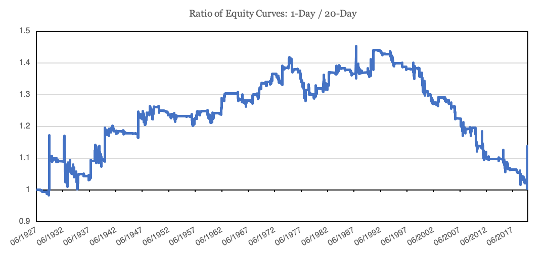
Source: Tiingo data. Calculations by Newfound Research.
We see a very interesting regime change: trading the signal immediately appeared to out-perform the 20-day tranche until the early 1990s, at which point tranching dramatically out-performed immediate implementation. At least until March 2002.
One potential argument for this regime shift is limits to arbitrage. Prior to the 1990s, actually implementing this trend equity strategy may have been near impossible or too costly. For example, it would have been difficult to efficiently trade an entire basket of equities back in the 1940s and 1950s. This could lead to short-term autocorrelation in hypothetical index returns that show up when we backtest, but only because they were not actually exploitable in practice!
Couple more efficient index access with lower trading costs and we may see a decrease in short-term autocorrelation that lead to a regime favoring tranching.
Or, perhaps, this was only an effect in U.S. equities. So, let’s plot this same ratio for a random cross-section of different asset classes, country indices, and equity sectors (using ETF proxies).
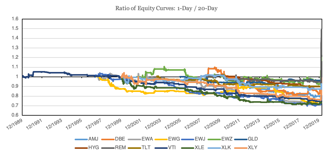
Source: Tiingo data. Calculations by Newfound Research.
Even including March 2020, only 2 of the 14 asset classes (mortgage REITs and Brazilian equities) ended up better off implementing immediately versus a 20-day tranche, and all the asset classes were worse off when measured prior to March.
Of course, these choices are not black-or-white. There is no reason we could not choose another tranching period (e.g. two weeks) or even diversify across tranching periods!
The Response Function
At the risk of getting unnecessarily technical, we can gain some insight into these tranching decisions by looking at how much emphasis our choice puts on prior signal changes.
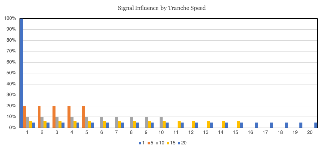
We can easily see that a 1-day tranche (i.e. immediate implementation) is influenced entirely by the prior day’s signal, whereas a 5-day tranche would be 20% weight on each of the last 5 days’ signals. A 20-day tranche puts 5% of the weight on each of the last 20 days.
But what happens if we start combining these? For example, what happens if we want 50% of our portfolio to respond immediately and 50% to respond over 20 days? Or 25% of our portfolio in 1-, 5-, 10-, and 20-day tranches? Or diversify equally across tranche speeds ranging from 1- to 20-days?
We can plot the response function weights below (note the change in y-axis scale).
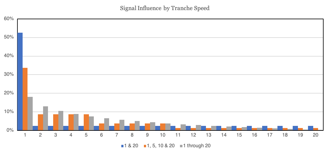
We can see that we can create non-linear response weights based upon these blends. For example, combining the 1- and 20-day tranches creates a sudden jump in weight after one day, whereas an equal-weight combination of 1- through 20-day tranche models creates a smoother influence curve.
The trade-off, of course, is that the smoother influence curve has less weight on the most recent signal than the blend that over-weights the 1-day tranche model.
But what these graphs tell us is that we can actually combine different tranching speeds to create response functions that we believe align better with our portfolio objectives or the prevailing market regime.
Conclusion
In this research note, we explored both the philosophical and empirical evidence behind tranching with trend models. Philosophically, the approach of implementing the signal incrementally over time can (1) help align portfolio construction with optimal forecast horizons, (2) potentially reduce impacts of whipsaw, and (3) modulate portfolio conviction based upon signal consistency over time.
Empirically, we found that prior to the 1990s, the immediate application of signals was superior to the tranching approach in U.S. equities. After the 1990s, a 20-day tranche significantly outperformed. Using a random cross-section of asset classes, we find that this evidence is not limited to U.S. equities.
As with most portfolio choices, these tranching decisions need not be black and white. In the final section of this note, we demonstrated that the decisions can be thought of as weighting schemes and that by diversifying across different tranching decisions we can construct different weighting approaches.
Related: The COVID-19 Impact on Retirement Savings of Americans